Mixed fisheries projections with FLasher
Finlay Scott, Iago Mosqueira - European Commission Joint Research Center
08 February, 2018
## Warning: replacing previous import 'ggplot2::%+%' by
## 'FLCore::%+%' when loading 'ggplotFL'
1 Introduction
In this vignette we demonstrate how FLasher can be used to simulate a mixed fishery, with multiple fisheries catching multiple stocks.
The vignette uses a simple mixed fishery case study, based on two fishing fleets catching European plaice (Pleuronectes platessa) and common sole (Solea solea). Projections of the fishery are performed under different management options, including economic metrics. Plaice and sole are two species that are commonly caught together, for example in the North Sea. However, the case study presented here is not based on a real scenario and is used only to demonstrate how such a system can be modelled using FLasher. The two stocks are fished by a beam trawl fishery and a gillnet fishery. The selectivities and fishing effort of each fishery are independent of each other.
The model has an annual timestep (seasonal models will be considered in a separate vignette).
To perform mixed fishery projections it is necessary to use the FLBiol and FLFishery classes, instead of the FLStock objects (which is one of the main differences between using the older package FLash and FLasher). Projecting with FLBiol and FLFishery objects requires a little more setting up than projecting with an FLStock, in terms of the objects themselves and also in terms of the projection control object.
The main difference is that the projection method, fwd() takes an FLFisheries object and an FLBiols object as well as the fwdControl object. An FLFisheries object is basically a list of FLFishery objects and an FLBiols object is a list of FLBiol objects. Each FLFishery contains one or more FLCatch objects which catch from the FLBiol objects. Multiple FLCatch objects from different FLFishery objects can catch from the same FLBiol. The output of running fwd() in this way is a named list with the updated FLFisheries and FLBiols objects.
Projection targets can be set at different levels. For example, a catch target can be set at the FLCatch level (the catch of that particular FLCatch) or at the FLBiol level (the total catch from an FLBiol which may be fished by one or more FLCatch objects. This means that when setting the projection control it is necessary to describe which FLFishery, FLCatch and FLBiol that target is attributed to. A description of which target types can be attributed to which object type can be seen in the FLasher reference manual (type vignette(topic=“FLasher_reference”, package=“FLasher”)).
This is better described with examples, which make up this tutorial.
2 Useful functions
The following functions are used for plotting the output of the FLasher projections. They will evenutally be moved inside the package when they are better.
# Handy function to get F from OP from FLasher
getf <- function(op, fn = 1, cn = 1, bn = 1, age_range = c(2,
    6)) {
    # f = alpha * sel * effort
    flf <- op[["fisheries"]][[fn]]
    flc <- flf[[cn]]
    b <- op[["biols"]][[bn]]
    f <- ((flc@catch.q[1, ] * quantSums(b@n * b@wt)^(-1 * flc@catch.q[2,
        ])) * flf@effort) %*% flc@catch.sel
    fbar <- apply(f[age_range[1]:age_range[2], ], 2:6, mean)
    return(fbar)
}

getrevcatch <- function(catch) {
    return(quantSums(catch@price * catch@landings.n * catch@landings.wt))
}

getrev <- function(fishery, catch = NA) {
    if (is.na(catch)) {
        # get all catches
        revs <- lapply(fishery, function(x) getrevcatch(x))
        rev <- Reduce("+", revs)
    } else {
        rev <- getrevcatch(fishery[[catch]])
    }
    return(rev)
}

# Plotting functions
plot_biomass <- function(biol, stock_name, years = 2:20) {
    tb <- c(quantSums(biol@n * biol@wt)[, ac(years)])
    plot(years, tb, type = "l", xlab = "Year", ylab = "Biomass",
        main = paste(stock_name, " biomass", sep = ""))
}

plot_catch <- function(biol_no, op, FCB, stock_name, years = 2:20,
    legpos = "topleft") {
    fcbf <- FCB[FCB[, "B"] == biol_no, , drop = FALSE]
    partialc <- list()
    for (i in 1:nrow(fcbf)) {
        catch_name <- names(op[["fisheries"]][[fcbf[i, "F"]]])[fcbf[i,
            "C"]]
        partialc[[catch_name]] <- c(catch(op[["fisheries"]][[fcbf[i,
            "F"]]][[fcbf[i, "C"]]])[, ac(years)])
    }
    totalc <- Reduce("+", partialc)
    minc <- min(unlist(lapply(partialc, min))) * 0.9
    maxc <- max(totalc) * 1.1
    colours <- c("blue", "red")
    plot(years, totalc, type = "l", xlab = "Year", ylab = "Catch",
        main = paste(stock_name, " catch", sep = ""), ylim = c(minc,
            maxc))
    if (length(partialc) > 1) {
        legend_names <- "Total"
        legend_cols <- "black"
        for (i in 1:length(partialc)) {
            lines(years, partialc[[i]], col = colours[i])
            legend_names <- c(legend_names, names(partialc)[i])
            legend_cols <- c(legend_cols, colours[i])
        }
        legend(legpos, legend = legend_names, col = legend_cols,
            lty = 1)
    }
}

plot_f <- function(biol_no, op, FCB, stock_name, years = 2:20,
    legpos = "topleft") {
    fcbf <- FCB[FCB[, "B"] == biol_no, , drop = FALSE]
    partialf <- list()
    for (i in 1:nrow(fcbf)) {
        catch_name <- names(op[["fisheries"]][[fcbf[i, "F"]]])[fcbf[i,
            "C"]]
        partialf[[catch_name]] <- c(getf(op, fn = fcbf[i, "F"],
            cn = fcbf[i, "C"], bn = biol_no)[, ac(years)])
    }
    totalf <- Reduce("+", partialf)
    minf <- min(unlist(lapply(partialf, min))) * 0.9
    maxf <- max(totalf) * 1.1
    colours <- c("blue", "red")
    plot(years, totalf, type = "l", xlab = "Year", ylab = "F",
        main = paste(stock_name, " F", sep = ""), ylim = c(minf,
            maxf), col = "black")
    if (length(partialf) > 1) {
        legend_names <- "Total"
        legend_cols <- "black"
        for (i in 1:length(partialf)) {
            lines(years, partialf[[i]], col = colours[i])
            legend_names <- c(legend_names, names(partialf)[i])
            legend_cols <- c(legend_cols, colours[i])
        }
        legend(legpos, legend = legend_names, col = legend_cols,
            lty = 1)
    }
}

plot_revenue <- function(fisheries, years = 2:20, legpos = "topleft") {
    nf <- length(fisheries)
    revs <- list()
    for (i in 1:nf) {
        revs[[i]] <- c(getrev(fisheries[[i]])[, ac(years)])
    }
    minr <- min(unlist(lapply(revs, min))) * 0.9
    maxr <- max(unlist(lapply(revs, max))) * 1.1
    colours <- c("blue", "red")
    plot(years, revs[[1]], type = "l", ylim = c(minr, maxr),
        xlab = "Year", ylab = "Revenue", main = "Fishery revenue",
        col = colours[1])
    if (length(revs) > 1) {
        legend_names <- names(fisheries)[1]
        legend_cols <- colours[1]
        for (i in 2:length(revs)) {
            lines(years, revs[[i]], col = colours[i])
            legend_names <- c(legend_names, names(fisheries)[i])
            legend_cols <- c(legend_cols, colours[i])
        }
        legend(legpos, legend = legend_names, col = legend_cols,
            lty = 1)
    }
}

plot_effort <- function(fisheries, years = 2:20, legpos = "topleft") {
    nf <- length(fisheries)
    eff <- list()
    for (i in 1:nf) {
        eff[[i]] <- c(fisheries[[i]]@effort[, ac(years)])
    }
    mine <- min(unlist(lapply(eff, min))) * 0.9
    maxe <- max(unlist(lapply(eff, max))) * 1.1
    colours <- c("blue", "red")
    plot(years, eff[[1]], type = "l", ylim = c(mine, maxe), xlab = "Year",
        ylab = "Effort", main = "Fishery relative effort", col = colours[1])
    if (length(eff) > 1) {
        legend_names <- names(fisheries)[1]
        legend_cols <- colours[1]
        for (i in 2:length(eff)) {
            lines(years, eff[[i]], col = colours[i])
            legend_names <- c(legend_names, names(fisheries)[i])
            legend_cols <- c(legend_cols, colours[i])
        }
        legend(legpos, legend = legend_names, col = legend_cols,
            lty = 1)
    }
}
3 The operating model
The full operating model comprises 2 fisheries (a beam trawl and a gillnet) fishing on two biological stocks (plaice and sole). The example is based on Scott and Mosqueira (2016). As mentioned above, although the example is based on a plaice and sole mixed fishery, it is not intended to represent any particular real-world example. The operating model only has one iteration for clarity.
The objects have already been created and are in the FLasher package. They are loaded here:
data(mixed_fishery_example_om)The data set contains two objects: biols (an FLBiols object containing an FLBiol each for plaice and sole) and flfs (an FLFisheries object containing an FLFishery each for the beam trawl and gillnet fisheries).
3.1 Exploring the biological stocks
The plaice and sole stocks are based on the life history of plaice and sole in the North Sea. They are each stored as FLBiol objects in a FLBiols list called biols. They can be accessed using the [[ operator, either by name or position.
The stock-recruitment (SR) models have been set using the _@rec_ slot of the FLBiol objects. Both stocks have Ricker SR models that are already parameterised:
# Plaice
biols[["ple"]]@rec
## An object of class "FLQuants": EMPTY
## model:
## rec ~ a * ssb * exp(-b * ssb)
## <environment: 0xaae7ff8>
##
## params:
## An object of class "FLPar"
## params
## a b
## 4.83e+00 1.33e-06
## units: NAbiols[["sol"]]@rec## An object of class "FLQuants": EMPTY
## model:
## rec ~ a * ssb * exp(-b * ssb)
## <environment: 0xaafc108>
##
## params:
## An object of class "FLPar"
## params
## a b
## 7.73e+00 2.75e-05
## units: NAThe SR models look like this:
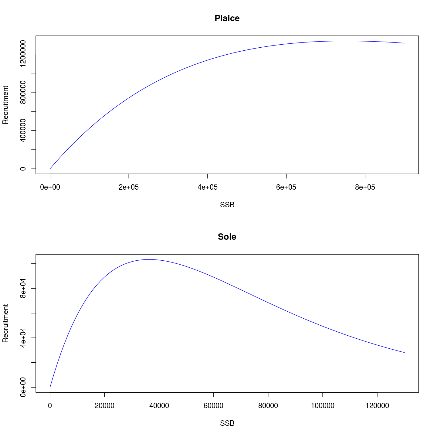
The stock-recruitment relationships of the plaice and sole stocks
Both biological stocks have 20 years. Only the first year has abundances. The other years will be filled in with the projected values.
3.2 Exploring the fisheries
There are two fisheries, a gillnet and a beam trawl, each stored as an FLFishery object, held in the FLFisheries list object, biols. Each fishery has 2 FLCatches, one that catches plaice and the other that catches sole.
The FLFishery objects can be accessed from the FLFisheries object by the [[ operator, either by name or position. It’s like accessing elements of a list. Each FLCatch within an FLFishery is also accessed by the [[ operator by name or position. Again, it’s like accessing elements of a list.
Each FLCatch has a selectivity pattern (stored in the catch.sel slot) and a catchability parameter (stored in the catch.q slot) depending on the gear type and the stock that is being caught.
The selectivities could be set by looking at the partial fishing mortalities or partial catches of each fishery if the data was available. Here we assume that the beam trawl has a logistic selection pattern and the gillnet has a dome shaped selection pattern. The selectivity patterns are assumed to be constant in time (although this does not have to be the case).
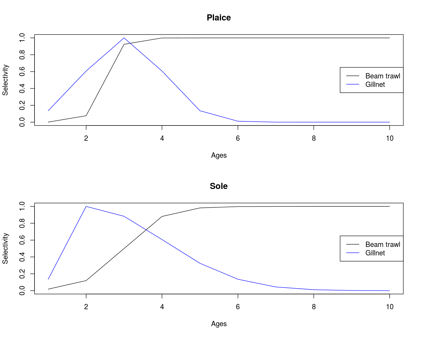
Selection patterns for the beam trawl (black) and gillnet (blue) fisheries on sole and plaice.
The catchability parameter, α, for each FLCatch links the fishing effort to the fishing mortality through the selection pattern. The partial F of each FLCatch on the stock is given by:
pFf,c,b=αf,c∗self,c∗effortf
where f, c and b are the fishery, catch and biological stock respectively.
Note that fishing effort is set at the fishery level (in the _@effort_ slot). Fishing effort is the only independent variable over which managers have any control. All other measures (landings, fishing mortality etc) are driven by the fishing effort. In all of the projections, the targets are hit by finding the fishing effort of each fishery in the projection.
Here the α parameter of each FLCatch has been set so that an effort of 1 from each fishery yields a mean F on each stock of 0.3. All of the projected effort values can then be considered as relative to this effort rather than an as absolute fishing effort. Here we assume that the catchability of the beam trawl gear is twice that of the gillnet.
Some prices have been added to the FLCatches to allow revenues to be calculated. Sole is assumed to be 5 times as expensive as plaice.
4 A note about target setting, independent variables and precedence of constraints
As mentioned above the independent variables in the projections are the efforts of each FLFishery in each time step. For a projection to make sense the number of independent variables must equal the number of dependent variables. This means that when there is more than one FLFishery there is more than one independent variable in each timestep and so there must be more than one target in each timestep. These targets are solved simultaneously.
For example, if we have two FLFishery objects we must set two targets per time step. These two targets are solved simultaneously, not one at a time. The two targets can be thought of as subtargets of a single target.
It is possible to set multiple targets. However, it is necessary that each target contains a number of subtargets, equal to the number of FLFishery objects, that are solved simultaneously. If we have two FLFishery objects, we can have multiple targets, but they must come in pairs that can be solved together.
Essentially, projecting a target in a time step is the same as solving a set of simultaneous equations. In the same way to solve a system of simultaneous equations the equations must be dependent on a mix all of the independent variables, the subtargets in each target must depend on a mix of the efforts from each FLFishery (it is not necessary for every subtarget to be dependent on each FLFishery).
The order of the targets in each timestep is important. The targets that are solved later have precedence over the ones solved earlier, i.e. solving a later target will essentially overwrite the results from the preceeding targets.
Constraint targets (minimum and maximum values) are solved last in each timestep. Internally, the non-constraint targets are solved first. The resulting status of the fisheries and stocks is then checked against the constraints. If the constraints have been breached, a second projection is then solved with the contraints as the targets. In this way the target constraints have the highest precedence.
Hopefully some of this will become clear in the examples.
5 Example: A single fishery and a single stock
Before we do anything complicated, we show a simple example with only a single fishery (the beam trawl) catching a single stock (plaice). This gives us a single independent variable (the fishing effort) to solve in each timestep (year). As described above, we only need to provide a single target for each timestep. In this example we project with a constant catch for all years.
First we make the simple fishery and biology objects based on the ones created above. Note that it is important that all FLFishery objects have an initial value for effort in the projection years. It cannot be 0 and it cannot be NA.
# First pull out a single FLCatch from the BT fishery using
# [[]]
pleBT <- flfs[["bt"]][["pleBT"]]
# Make a single beam trawl FLFishery with 1 FLCatch
bt1 <- FLFishery(pleBT = pleBT)
# Set the initial effort
bt1@effort[] <- 1
# Make an FLFisheries from it
flfs1 <- FLFisheries(bt = bt1)
# Make an FLBiols with a single FLBiol
biols1 <- FLBiols(ple = biols[["ple"]])
In this first example we set a constant total catch target for 20 years (we assume that there is no fishing in year 1). We set a projection control object to reflect this.
In the contol object we need to specify to which object the catch target is related to. This is a key difference between projecting FLasher with an FLStock and with an FLBiols and FLFisheries. In this example, the catch target relates to the total catch from the FLBiol. We therefore use the biol column to specify this. This column takes either an integer to specify the position of the chosen FLBiol in the FLBiols list, or, more conveniently, the name of the FLBiol in the FLBiols list. In this case we only have one FLBiol in the FLBiols object so the entry in the biol column could be 1. Alternatively, as we have named the FLBiol objects, we could also set the biol column to the name ple.
Another difference between projecting FLasher with an FLStock and with an FLBiols and FLFisheries is the need to specify the FCB matrix to describe what FLCatch from what FLFishery is fishing on what FLBiol. The FCB matrix always has three columns: F, C and B which describe the positions of the FLFishery objects within the FLFisheries object, the position of the FLCatch objects in the FLFishery objects, and the position of the FLBiol objects in the FLBiols object. It is essentially a map of what is fishing on who. In this example, we only a single FLBiol that is being fished by the only FLCatch of the only FLFishery. Hence the FCB matrix only one row, all filled with 1s. The FCB matrix looks like this which means that the first FLCatch of the FLFishery is catching from the first FLBiol:
fcb <- matrix(1, nrow = 1, ncol = 3, dimnames = list(1, c("F",
    "C", "B")))
fcb
## F C B
## 1 1 1 1To make the control object we can either pass a data.frame or a list to the fwdControl() method. Here we pass a data.frame.
catch_target <- 1e+05
flasher_ctrl_target <- data.frame(year = 2:20, quant = "catch",
    biol = "ple", value = catch_target)
flasher_ctrl <- fwdControl(flasher_ctrl_target, FCB = fcb)
An alternative is to pass a named list. Using this method is easier for making complicated control objects (see later).
flasher_ctrl <- fwdControl(list(year = 2:20, quant = "catch",
    biol = "ple", value = catch_target), FCB = fcb)
We can draw the fishery system using the draw() method:
draw(flasher_ctrl, fisheryNames = "Beam", catchNames = "Plaice catch",
    biolNames = "Plaice")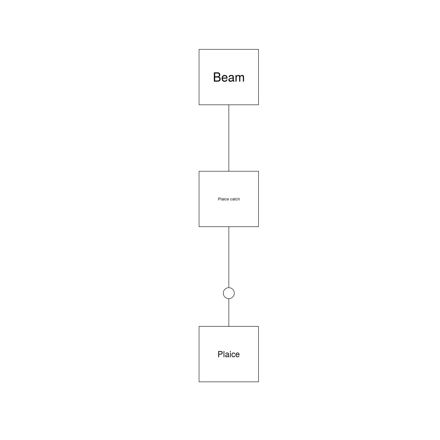
A single Fishery with 1 Catch fishing on a single Biol
We run the projection calling fwd() passing in the FLBiols, the FLFisheries and the control objects:
test <- fwd(object = biols1, fishery = flfs1, control = flasher_ctrl)The output from running fwd() with FLFisheries and FLBiols is a named list.
is(test)## [1] "list" "vector"names(test)## [1] "biols" "fisheries" "control" "flag"The contents of the output list are the updated FLFisheries and FLBiols objects, the fwdControl object and a mysterious other object called flag. flag is the output from the solver and is a matrix of integers indicating which targets, or subtarget, (rows) and iterations (columns) successfully solved and which didn’t. The number 1 indicates that target and iteration solved successfully. The number -1 indicates that the solver iterations maxed out. The numbers -2 and -3 indicate that the solver limits were breached.
Here we have 1 column as we only have 1 iteration. We have 19 rows as we have 19 targets (1 for each year). All the flags are 1 so all targets solved OK.
test[["flag"]]## [,1]
## [1,] 1
## [2,] 1
## [3,] 1
## [4,] 1
## [5,] 1
## [6,] 1
## [7,] 1
## [8,] 1
## [9,] 1
## [10,] 1
## [11,] 1
## [12,] 1
## [13,] 1
## [14,] 1
## [15,] 1
## [16,] 1
## [17,] 1
## [18,] 1
## [19,] 1We can see that the constant catch target has been hit in the target years. The plot also shows the resulting fishing mortality, relative effort, revenue of the fishery and biomass of the stock. The biomass is also driven by the stock-recruitment relationship of the stock and the initial dynamics will be affected by the initial age structure.
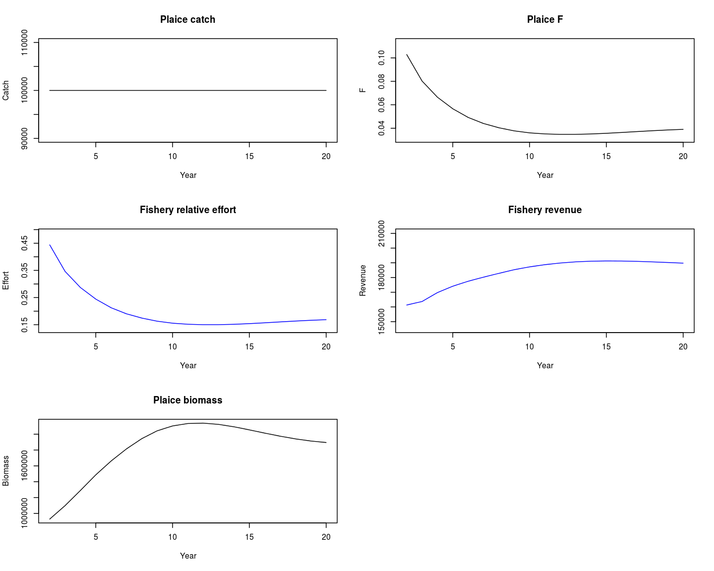
Summary results of projecting a single stock with a single fishery with a constant catch target.
6 Example: A single fishery with two stocks
Here, we build on the previous example and introduce the sole stock as an additional stock that will be caught by the same fishery. The FLFishery object will now contain two FLCatch objects which catch plaice and sole respectively. The FLBiols object will have two FLBiol objects: plaice and sole. We still only have one fishery (the beam trawl, constructed above) so we still have only one independent variable (the fishing effort) in each year. The same fishing effort is applied to both stocks as they are caught by the same fishery.
# Extract the beam trawl fishery from the FLFisheries loaded
# above
bt <- flfs[["bt"]]
# Create a new FLFisheries with the single FLFishery
flfs2 <- FLFisheries(bt = bt)
# It has only one FLFishery
length(flfs2)
## [1] 1# That FLFishery has 2 FLCatches
length(flfs2[["bt"]])## [1] 2# The FLBiols has 2 FLBiol objects
length(biols)## [1] 2# The names of the FLBiol objects are
names(biols)## [1] "ple" "sol"As we have only one independent variable (effort from one FLFishery) we cannot set a catch target for each stock (i.e. two dependent variables) because that would require two independent variables. Additionally, the catches of the two stocks are of course linked as they are caught by the same fishery. This means that we do not have the freedom to hit independent catch targets at the same time. This is a typical mixed fishery problem.
In this first example we set only a catch target for the plaice stock. We again use the biol column to specify which FLBiol the catch target relates to. There are two FLBiol objects in the FLBiols object. We saw above that the first one is the plaice stock and the second one is the sole stock. This means that to apply the catch target to the plaice stock we could put 1 or “ple” in the biol column. If we wanted to apply the catch target to the sole stock we would put “sol” or 2.
This example requires a slightly more complicated FCB matrix. It reflects that we have one fishery with two catches, each catching a different stock. Again, the numbers in the columns reflect the positions of the objects in their lists. Here, the first FLCatch of the first (only) FLFishery catches from the first FLBiol and the second FLCatch of the first (only) FLFishery catches from the second FLBiol.
We make the control object using the list based constructor:
fcb <- matrix(c(1, 1, 1, 2, 1, 2), nrow = 2, ncol = 3, dimnames = list(1:2,
    c("F", "C", "B")))
plaice_catch_target <- 250000
flasher_ctrl <- fwdControl(list(year = 2:20, quant = "catch",
    biol = "ple", value = plaice_catch_target), FCB = fcb)
The FCB matrix looks like this:
flasher_ctrl@FCB## F C B
## 1 1 1 1
## 2 1 2 2Take a look at the fishery system:
draw(flasher_ctrl, fisheryNames = "Beam trawl", catchNames = c("Ple catch",
    "Sol catch"), biolNames = c("Ple", "Sol"))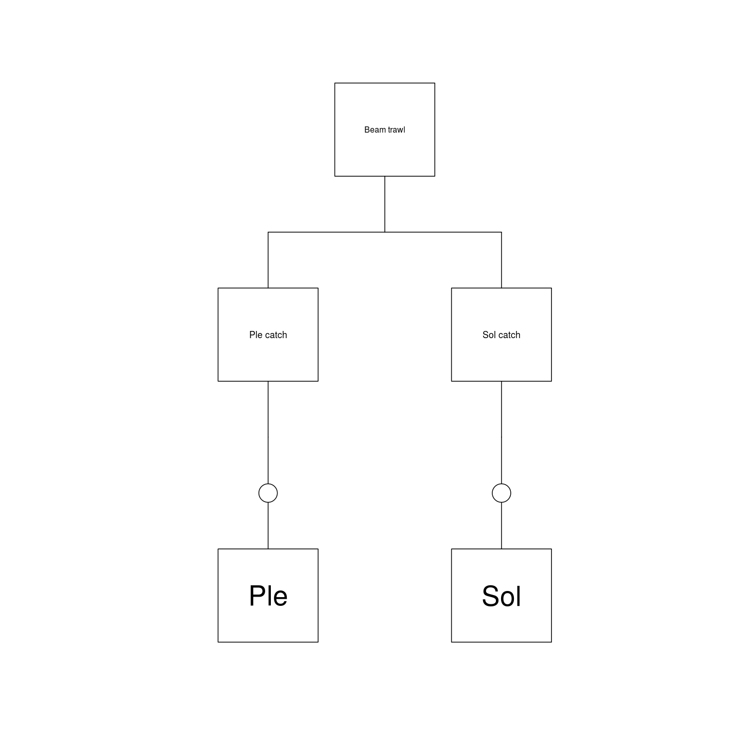
A single Fishery with 2 Catches, each fishing on a single Biol
And project:
test <- fwd(object = biols, fishery = flfs2, control = flasher_ctrl)We can see that the plaice catch target has been hit. We also look at the resulting sole catches, Fs, relative effort, revenue and biomasses that resulted from fishing at the effort that yielded the plaice target catch.
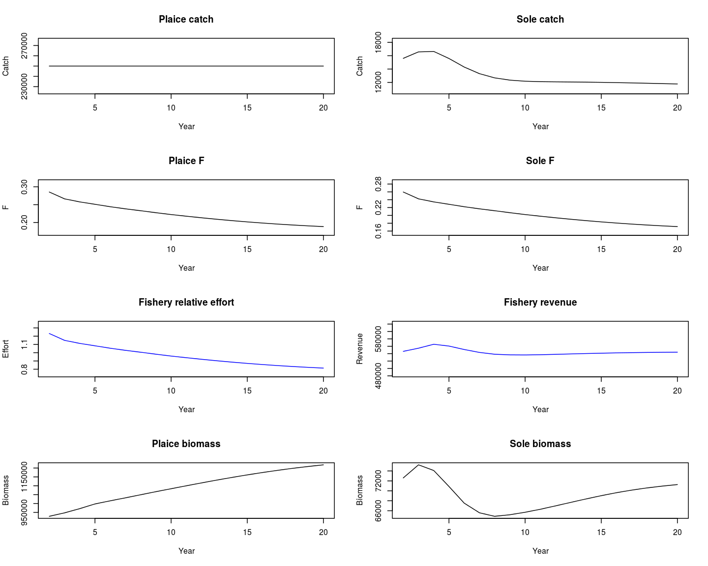
Summary results of projecting two stocks with a single fishery with a constant catch target on plaice.
As mentioned above, we cannot also have a target for the sole catch that is hit simultaneously as the plaice catch target. However, we can add a limit to the amount of fishing pressure that sole is subject to. For example, we can set a maximum F for sole.
We saw in the last example that catching the plaice catch target results in a maximum F for sole of about 0.26. We can set a limit of maximum F of 0.2 (this number is made up for the sake of the example).
In this control object we set a catch target for biol = “ple” (plaice) and also an F target for biol = “sol” (sole). When setting an F target it is necessary to specify the minimum and maximum ages of the Fbar range. This information is automatically taken from the FLStock when projecting with an FLStock. However, an FLBiol does not have this information and so it must be supplied in the control object in the minAge and maxAge columns. When setting the sole target instead of setting a value we set a max.
We again make use of the list creator for the fwdControl. This is convenient as we can pass a list for each of the targets we are trying to hit. This time we pass in two lists, one to set the plaice target, the other for the sole target.
plaice_catch_target <- 250000
sole_f_limit <- 0.2
flasher_ctrl <- fwdControl(list(year = 2:20, quant = "catch",
    biol = "ple", value = plaice_catch_target), list(year = 2:20,
    quant = "f", biol = "sol", max = sole_f_limit, minAge = 2,
    maxAge = 6), FCB = fcb)
test <- fwd(object = biols, fishery = flfs2, control = flasher_ctrl)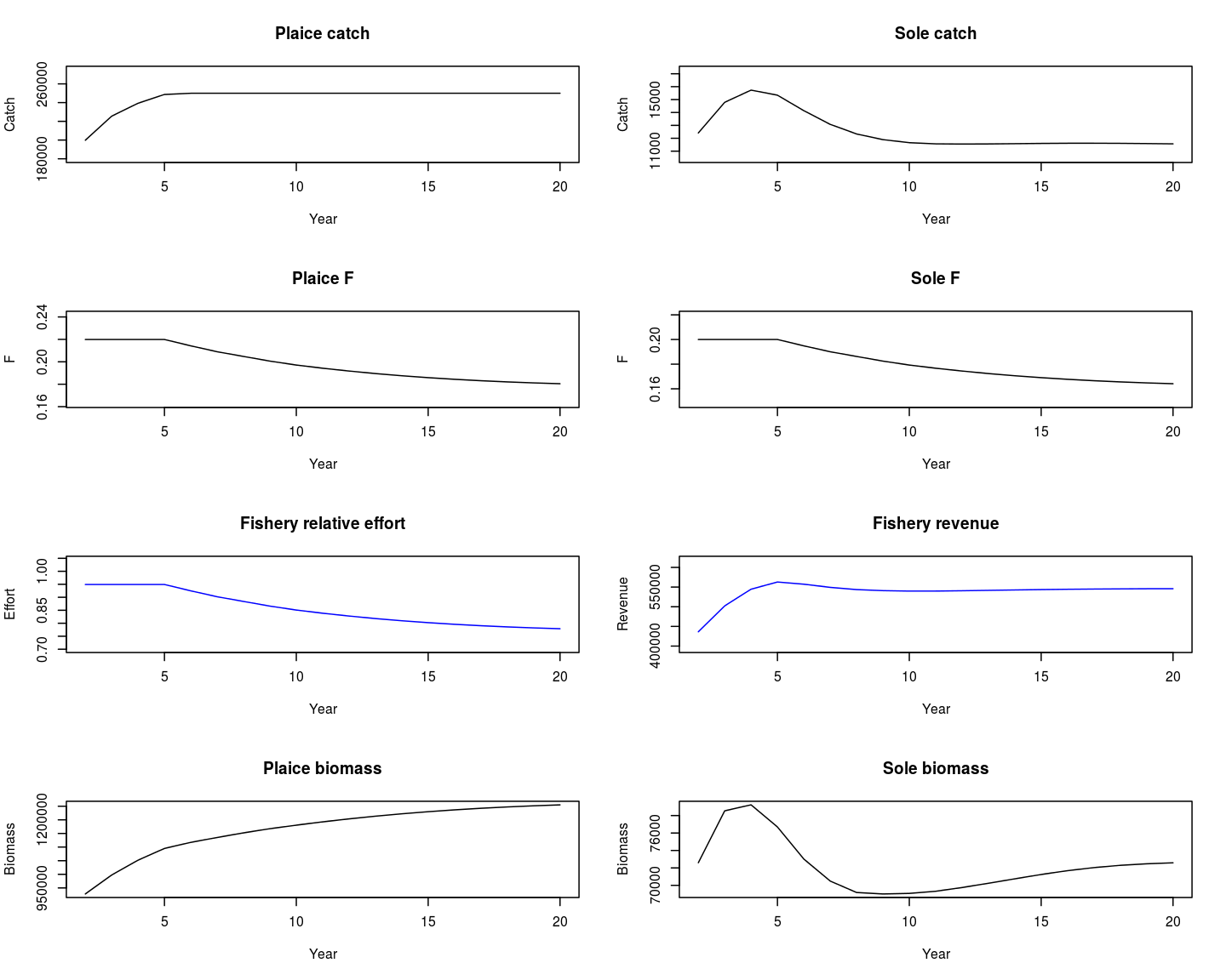
Summary results of projecting two stocks with a single fishery with a constant catch target on plaice and a maximum F limit on sole.
We can see that the maximum limit of F on sole has come into effect at the start of the projection and continues until year 5. The catches on plaice in those years has been limited and the target plaice catch has not been hit. After year 5, the required fishing effort to catch the plaice target is sufficiently low that the resulting F on sole is less than 0.2. This demonstrates how FLasher can be used to simulate management decisions on a fishery that fishes multiple stocks.
7 Example: Two fisheries on a single stock
In this example we simulate two different fisheries (beam trawl and gillnet) that are fishing the same stock (sole). The FLFisheries will have two FLFishery objects, each with one FLCatch which fish on sole. The FLBiols object will have a single FLBiol (sole). We make the FLFishery and FLBiol objects like this (initial effort has been set to 1):
# Two fisheries on a single stock Make the plaice fishery
# with a single FLCatch
bt3 <- FLFishery(solBT = flfs[["bt"]][["solBT"]], desc = "")
bt3@effort[] <- 1
# Make the sole fishery with a single FLCatch
gn3 <- FLFishery(solGN = flfs[["gn"]][["solGN"]], desc = "")
gn3@effort[] <- 1
# Make the FLFisheries
flfs3 <- FLFisheries(bt = bt3, gn = gn3)
# Make the FLBiols with a single FLBiol
biols3 <- FLBiols(sol = biols[["sol"]])
We have two fisheries which means we have two independent variables (the effort from each of the fisheries) to manipulate to hit the targets. This means that we cannot set just a single target in each timestep, e.g. we cannot only set a target for the total catch of sole because there are an infinite number of ways that the two effort levels can be set to hit the total catch. It is necessary to set two subtargets per timestep which will be solved simultaneously.
7.1 Two catch subtargets
A first example is to set target catches for each of the fisheries (a target catch for sole caught by the beam trawl and a target catch for sole caught by the gillnet) i.e. to set partial catches at the FLCatch level. For example, if the stock is managed by a single TAC, we can use the individual fishery quotas for targets.
Note that now the catch target is set at the FLFishery and FLCatch level, not the FLBiol level as in the previous examples. To do this we use the fishery and catch column to specify which FLFishery and FLCatch objects relate to the target. They can be specified by position in their lists (e.g. position of the FLCatch in the parent FLFishery) or by name. Here there is a catch target that relates to the first (only) FLCatch of the beam trawl FLFishery and another catch target that relates to the first (only) FLCatch of the gillnet FLFishery. The names of the FLFishery objects and their respective FLCatch objects are:
# Names of the FLFishery objects
names(flfs3)
## [1] "bt" "gn"# Names of their FLCatch objects
names(flfs3[["bt"]])## [1] "solBT"names(flfs3[["gn"]])## [1] "solGN"The biol column can now be ignored.
sole_bt_catch <- 10000
sole_gn_catch <- 5000
fcb <- matrix(c(1, 2, 1, 1, 1, 1), nrow = 2, ncol = 3, dimnames = list(1:2,
    c("F", "C", "B")))
flasher_ctrl <- fwdControl(list(year = 2:20, quant = "catch",
    fishery = "bt", catch = "solBT", value = sole_bt_catch),
    list(year = 2:20, quant = "catch", fishery = "gn", catch = "solGN",
        value = sole_gn_catch), FCB = fcb)
Note that the FCB matrix has been changed to reflect the relationship between the objects. The first (only) FLCatch of the first FLFishery catches from the first (only) FLBiol and the first (only) FLCatch of the second FLFishery also catches from the first (only) FLBiol
flasher_ctrl@FCB## F C B
## 1 1 1 1
## 2 2 1 1Take a look at the fishery system:
draw(flasher_ctrl, fisheryNames = names(flfs3), catchNames = unlist(lapply(flfs3,
    names)), biolNames = names(biols3))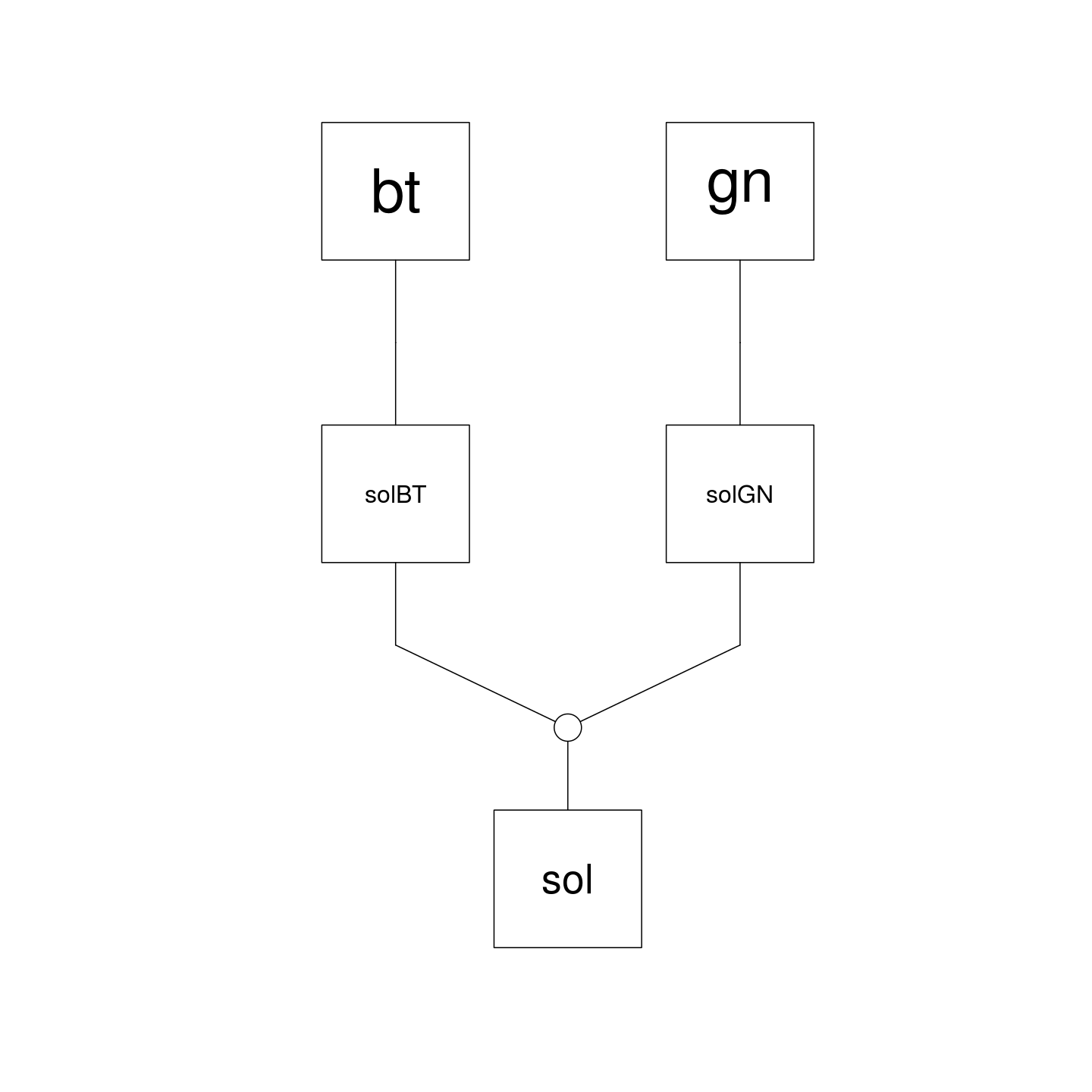
Two Fisheries with one Catch each fishing on a single Biol
And project:
test <- fwd(object = biols3, fishery = flfs3, control = flasher_ctrl)Both catch targets been hit although this has resulted in increasing fishing mortality on the stock. The plot also shows the partial fishing mortality from each fishery and it can be seen that the most of the fishing mortality comes from the beam trawl fishery. The beam trawl also also has a correspondingly higher revenue even though the relative effort is not higher (suggesting the profit will be higher, something which can be explored when further economic indicators are added to FLasher).
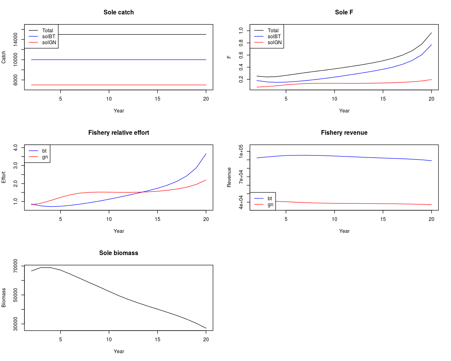
Summary results of projecting one stock with two fisheries with a constant catch target on both fisheries
We can also check if each pair of subtargets have been hit by looking at the flag element of the fwd() output:
test[["flag"]]## [,1]
## [1,] 1
## [2,] 1
## [3,] 1
## [4,] 1
## [5,] 1
## [6,] 1
## [7,] 1
## [8,] 1
## [9,] 1
## [10,] 1
## [11,] 1
## [12,] 1
## [13,] 1
## [14,] 1
## [15,] 1
## [16,] 1
## [17,] 1
## [18,] 1
## [19,] 1We have 19 targets (one of each year) and each target is made up of the two subtargets. A one means that the target was hit.
7.2 Absolute and relative catches
An alternative approach is to set a total catch at the stock level (for example, if the stock was managed through a TAC) and set an accompanying relative catch between the fisheries (for example, to maintain the historic relative stability of the fleets). In this way we do not explicitly specify how much the fisheries will catch, only that the total must be equal to the TAC and the historic relative stability must be respected.
This is quite a complicated control object! Here we set a total catch target of the stock to be 12000 and also that the catch of the beam trawl fishery is twice that of the gillnet. We again set two targets. The first specifies the total catch from the sole stock and requires the use of the biol column. The second specifies the relative catch of the two FLCatch objects in the two FLFishery objects. This involves the use of the relFishery and relCatch columns to describe the total catch relative to another fishery. Here we are saying the catch of the solBT FLCatch of the bt FLFishery in the FLFisheries object is relative to the solGN FLCatch of the gn FLFishery object. As we are setting a relative target, we also need to specify the relative year in which we hit the target using the relYear column.
We make the fwdControl object by passing a list for each subtarget. One of the targets is relative, hence all the additional elements. In each timestep the two subtargets will be solved simultaneously.
sole_catch_target <- 12000
sole_bt_gn_catch_relative <- 2
flasher_ctrl <- fwdControl(list(year = 2:20, quant = "catch",
    biol = "sol", value = sole_catch_target), list(year = 2:20,
    quant = "catch", relYear = 2:20, fishery = "bt", catch = "solBT",
    relFishery = "gn", relCatch = "solGN", value = sole_bt_gn_catch_relative),
    FCB = fcb)
test <- fwd(object = biols3, fishery = flfs3, control = flasher_ctrl)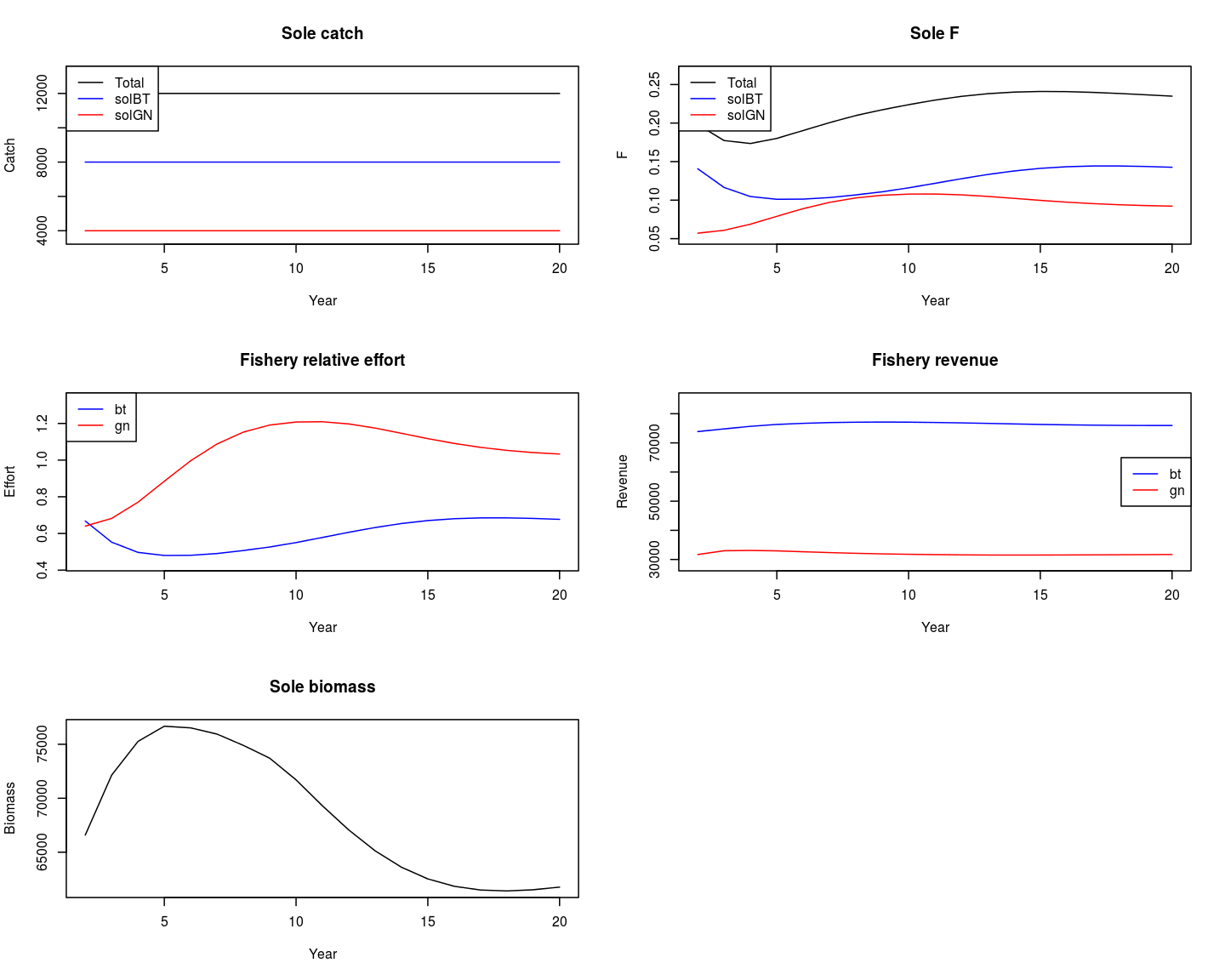
Summary results of projecting one stock with two fisheries with a constant total catch target and relative catch
We can see that the relative catch target between the fisheries has been hit. Also, the total catches from both fisheries is the same as the total catch target on the FLBiol.
8 Example: a mixed fishery
In this example we have a full mixed fishery consisting of two fisheries (a beam trawl and a gill net) each of which catch from two stocks (plaice and sole).
As above, we have two independent variables (the fishing effort of the two fisheries) so we need to set 2 subtargets for each target. However, there is no guarantee that the targets can be met. For example, setting a very low total catch of sole and a high total catch of plaice cannot be achieved simultaneously because catching plaice means sole are also caught.
8.1 Bad example with two catch targets
In this example we try to do the impossible which is hit an catch target for each of the stocks. However, given the interactions between catching the stocks this is not possible.
fcb <- matrix(c(1, 1, 1, 1, 2, 2, 2, 1, 1, 2, 2, 2), byrow = TRUE,
    ncol = 3, dimnames = list(1:4, c("F", "C", "B")))
sole_catch_target <- 12000
plaice_catch_target <- 5000
flasher_ctrl <- fwdControl(list(year = 2:20, quant = "catch",
    biol = "sol", value = sole_catch_target), list(year = 2:20,
    quant = "catch", biol = "ple", value = plaice_catch_target),
    FCB = fcb)
The FCB matrix has been updated to reflect the complicated mixed fishery:
flasher_ctrl@FCB## F C B
## 1 1 1 1
## 2 1 2 2
## 3 2 1 1
## 4 2 2 2Take a look at the fishery system:
draw(flasher_ctrl, fisheryNames = names(flfs), catchNames = unlist(lapply(flfs,
    names)), biolNames = names(biols))
Two Fisheries, each with 2 Catches fishing on two Biols
And project:
test <- fwd(object = biols, fishery = flfs, control = flasher_ctrl)FLasher hasn’t complained or thrown an error which looks like maybe the projection ran OK. However, if we look at the solver flag we can see that the solver was unable to find a solution (it runs out of iterations, hence the -1 flag).
test[["flag"]]## [,1]
## [1,] -2
## [2,] -2
## [3,] -2
## [4,] -2
## [5,] -2
## [6,] -2
## [7,] -3
## [8,] -3
## [9,] -2
## [10,] -2
## [11,] -3
## [12,] -3
## [13,] -3
## [14,] -3
## [15,] -3
## [16,] -3
## [17,] -3
## [18,] -3
## [19,] -3Additionally, the catches of the two stocks show that the targets have not been hit.
catch(test[["fisheries"]][["bt"]][["pleBT"]]) + catch(test[["fisheries"]][["gn"]][["pleGN"]])## , , unit = unique, season = all, area = unique
##
## year
## age 1 2 3 4
## all 7.302 172659.253 229605.652 241473.832
## year
## age 5
## all 216375.836
##
## [ ... 10 years]
##
## year
## age 16 17 18 19
## all 4.1504e-06 4.1504e-06 4.1504e-06 4.1504e-06
## year
## age 20
## all 4.1504e-06catch(test[["fisheries"]][["bt"]][["solBT"]]) + catch(test[["fisheries"]][["gn"]][["solGN"]])## , , unit = unique, season = all, area = unique
##
## year
## age 1 2 3 4
## all 4.5258 21105.6081 23020.3874 21714.6572
## year
## age 5
## all 18881.8040
##
## [ ... 10 years]
##
## year
## age 16 17 18 19
## all 3.0296e-06 3.0296e-06 3.0296e-06 3.0296e-06
## year
## age 20
## all 3.0296e-068.2 Example with constant total sole catch
Sole is more valuable than plaice so it is assumed that the total TAC of sole will be taken at the expense of taking all of the plaice TAC (essentially forgoing the plaice catch to maximise the sole catch). Instead of including catch targets for both stocks, we can a use relative target for plaice catches based on the historic relative stability, i.e. if we take all of the sole TAC we don’t know what the eventual total catch of plaice will be but we want the relative catches of plaice between the fisheries to be fixed.
In this example we set a total sole catch (biol = “sol” in the control object). We also set a relative plaice catch between the fisheries. The “pleBT” FLCatch of the “bt” beam trawl FLFishery takes 1.5 times as much plaice as the “pleGN” FLCatch of the “gn” gillnet FLFishery.
sole_catch_target <- 12000
plaice_bt_gn_catch_relative <- 1.5

flasher_ctrl <- fwdControl(list(year = 2:20, quant = "catch",
    biol = "sol", value = sole_catch_target), list(year = 2:20,
    quant = "catch", relYear = 2:20, fishery = "bt", catch = "pleBT",
    relFishery = "gn", relCatch = "pleGN", value = plaice_bt_gn_catch_relative),
    FCB = fcb)
And project:
test <- fwd(object = biols, fishery = flfs, control = flasher_ctrl)The total sole catch target from both fisheries has been hit with the gillnet fishery taking more of it. The target of relative catches between the fisheries of plaice has also been hit. The beam trawl takes more plaice than the gillnet and this difference is enough to mean that the revenue of the beam trawl is higher than for the gillnet, despite the sole catches of the gillnet being higher than for the beam trawl. The relative effort of the gillnet fishery is also higher than for the beam trawl. Both stocks experience an increase followed by decrease in biomass (the dynamic being partly driven by the age structure of the initial population).
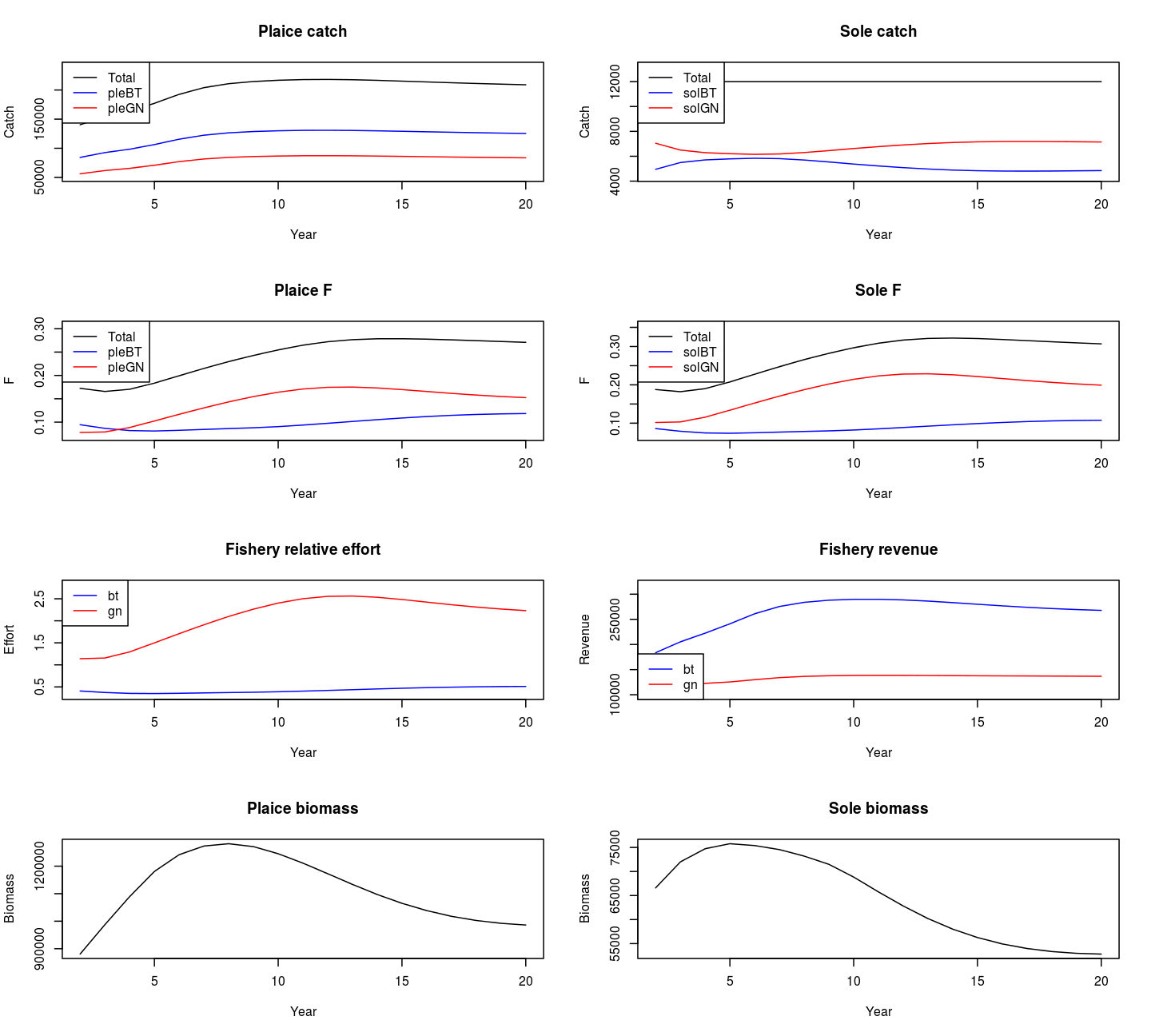
Summary results of projecting a mixed fishery with two stocks and two fleets with a constant total sole catch target and a relative plaice catch
8.3 A more complicated example with decreasing catches
In this more complicated example we set the total catch of sole in the first year, and then decrease it yearly to 90% of the previous year. We also set the relative plaice catch from the beam trawl to be 1.5 the catch from the gillnet.
This example makes extensive use of relative targets.
sole_catch_target_initial <- 20000
sole_catch_decrease <- 0.9
plaice_bt_gn_catch_relative <- 1.5

flasher_ctrl <- fwdControl(list(year = 2, quant = "catch", biol = "sol",
    value = sole_catch_target_initial), list(year = 3:20, quant = "catch",
    relYear = 2:19, biol = "sol", relBiol = "sol", value = sole_catch_decrease),
    list(year = 2:20, quant = "catch", relYear = 2:20, fishery = "bt",
        catch = "pleBT", relFishery = "gn", relCatch = "pleGN",
        value = plaice_bt_gn_catch_relative), FCB = fcb)
test <- fwd(object = biols, fishery = flfs, control = flasher_ctrl)
The sole catches have decreased by 0.9 each year. The plaice catches have also decreased but the relative catches between the fisheries remains constant. The biomass of both stocks increases rapidly whilst the revenue decreases along with the relative effort.
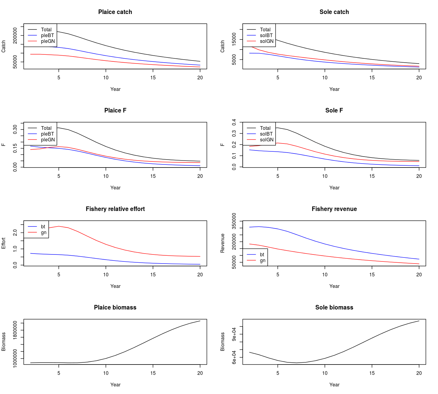
Summary results of projecting a mixed fishery with two stocks and two fleets with a decreasing total sole catch target and a relative plaice catch
9 Economic targets
The examples so far have focussed on setting catch and F targets. It is also possible to set the revenue as a target at either the catch level (for example, the revenue from the plaice portion of the beam trawl catch) or the fishery level (the sum of revenues from all the catches of that fishery). More economic indicators, such as costs and profits, will be added in the future.
We saw in the previous example that the revenues of both fisheries decreases as the sole catches decrease by 10% each year. Although, the stock biomasses increase, the decrease in revenue is likely to be unacceptable by the fishing industry. Given their costs of operation they may expect a minimum revenue, even if means the total catch exceeds the TAC.
To simulate this we can add a minimum revenue as a contraint target. As mentioned above, as we have two independent variables the targets must be supplied as pairs of subtargets. One pair of subtargets is the catch targets used above. In this example we add another pair of subtargets to each timestep. These subtargets are minimum revenues for each fishery. The target quant os “revenue”. Revenue is calculated at the FLFishery level meaning that only the FLFishery needs to be specified in the control object. This is a complicated projection. However, each target can be specified as a separate list to the fwdControl constructor to help organise it.
sole_catch_target_initial <- 20000
sole_catch_decrease <- 0.9
plaice_bt_gn_catch_relative <- 1.5
bt_min_revenue <- 150000
gn_min_revenue <- 1e+05

flasher_ctrl <- fwdControl(list(year = 2, quant = "catch", biol = "sol",
    value = sole_catch_target_initial), list(year = 3:20, quant = "catch",
    relYear = 2:19, biol = "sol", relBiol = "sol", value = sole_catch_decrease),
    list(year = 2:20, quant = "catch", relYear = 2:20, fishery = "bt",
        catch = "pleBT", relFishery = "gn", relCatch = "pleGN",
        value = plaice_bt_gn_catch_relative), list(year = 2:20,
        quant = "revenue", fishery = "bt", min = bt_min_revenue),
    list(year = 2:20, quant = "revenue", fishery = "gn", min = gn_min_revenue),
    FCB = fcb)
test <- fwd(object = biols, fishery = flfs, control = flasher_ctrl)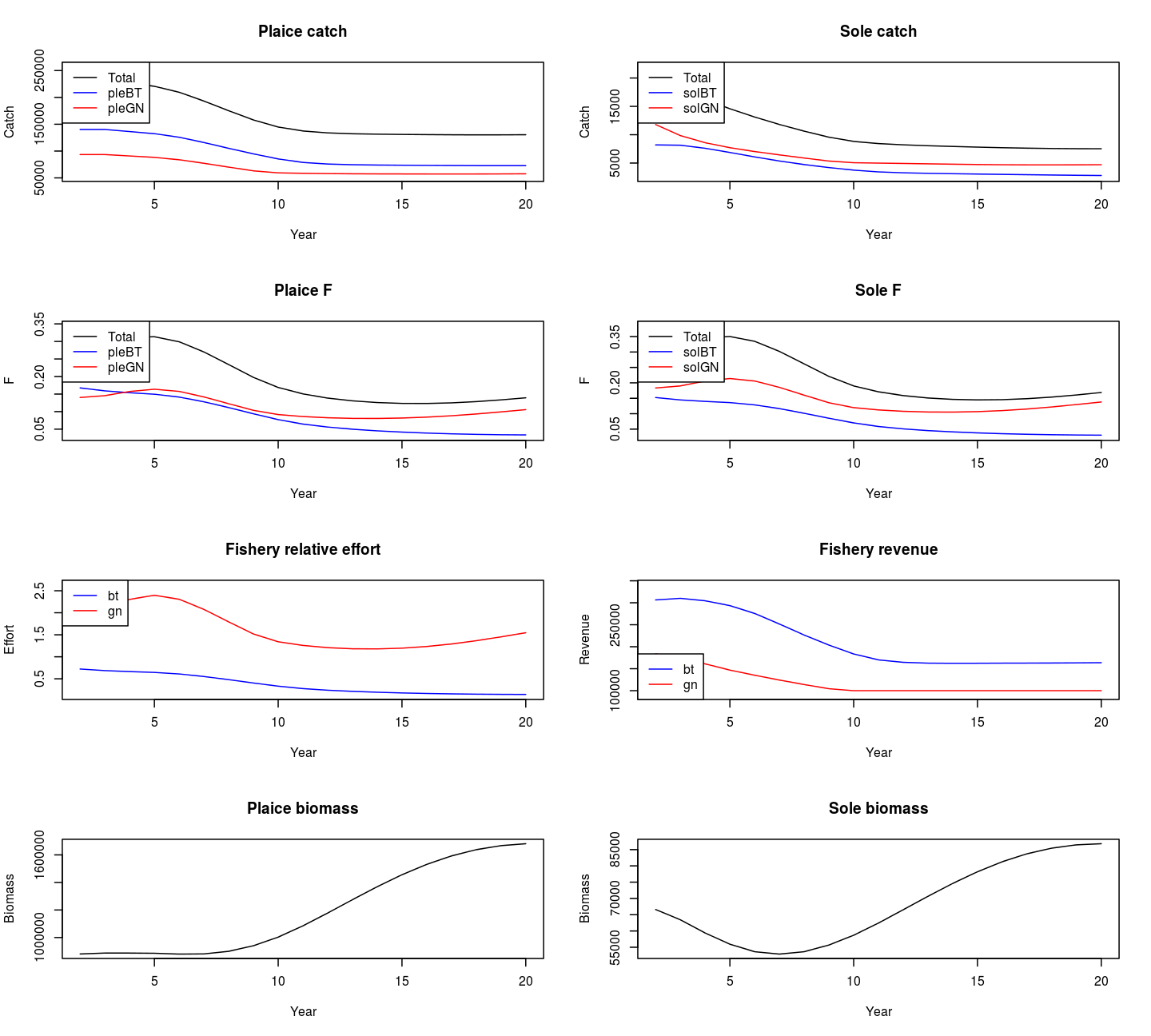
Summary results of projecting a mixed fishery with two stocks and two fleets with a decreasing sole catch target and a relative plaice catch. Minimum limits to the revenues of both fleets are also included.
What happened? We can see that the minimum revenue of the gillnet fishery comes into effect in year 10. After this year, the gillnet revenue hits the minimum level and does not decrease further. This has knock-on effects. From year 10, the annual decrease in sole catches is no longer 10% and the total sole catches remain approximately constant. The minimum revenue of the beam trawl fishery is never breached. With the limit on the sole revenue being reached, it is not possible to continue to hit the relative plaice catch targets between the fisheries (although it gets as close as possible).
10 Joint targets
FLasher can also be used to perform projections with joint targets. A joint target means a target that is the sum of metrics from more than one FLFishery or FLBiol object. For example, a combined species TAC (such as for dab and flounder in the North Sea) can be simulated by setting a joint catch target from more than one FLBiol.
10.1 Simple example with a combined species TAC
In this simple example we have a single beam trawl FLFishery with two FLCatch objects, each fishing on a single FLBiol (plaice and sole). We can set a catch target so that the total catch is the sum of the catches from each FLBiol.
# Extract the beam trawl fishery
bt <- flfs["bt"]
To make the control object we use the list-based constructor. To specify that a target is the sum of metrics from multiple objects we use the G() function. Here we specify a combined target for the two FLBiol objects, ple and sol. We project for the years 2 to 5 only.
joint_tac <- 2e+05
years <- 2:5
fcb <- matrix(c(1, 1, 1, 2, 1, 2), nrow = 2, ncol = 3, dimnames = list(1:2,
    c("F", "C", "B")))
ctrl <- fwdControl(list(year = years, quant = "catch", value = joint_tac,
    biol = G("ple", "sol")), FCB = fcb)
If we look at the control object we can see that the biol column has two names in it instead of just one. This means that the target applies to the sum of the catches of those stocks.
ctrl## An object of class "fwdControl"
## (step) year quant biol min value max
## 1 2 catch ple, sol NA 200000.000 NA
## 2 3 catch ple, sol NA 200000.000 NA
## 3 4 catch ple, sol NA 200000.000 NA
## 4 5 catch ple, sol NA 200000.000 NAWe project as normal:
test <- fwd(object = biols, fishery = bt, control = ctrl)We can check that the total catch from both the stocks is the same as the target:
# plaice catch
catch_ple <- catch(test[["fisheries"]][["bt"]][["pleBT"]])[,
    ac(years)]
# sole catch
catch_sol <- catch(test[["fisheries"]][["bt"]][["solBT"]])[,
    ac(years)]
catch_sol + catch_ple
## An object of class "FLQuant"
## , , unit = unique, season = all, area = unique
##
## year
## age 2 3 4 5
## all 2e+05 2e+05 2e+05 2e+05
##
## units: NAIn this example plaice makes up the majority of the catch.
catch_sol/(catch_sol + catch_ple)## An object of class "FLQuant"
## , , unit = unique, season = all, area = unique
##
## year
## age 2 3 4 5
## all 0.058429 0.061289 0.061256 0.057716
##
## units: NAcatch_ple/(catch_sol + catch_ple)## An object of class "FLQuant"
## , , unit = unique, season = all, area = unique
##
## year
## age 2 3 4 5
## all 0.94157 0.93871 0.93874 0.94228
##
## units: NAThe same effort is applied to each stock so the proportion in the total catch is determined by the abundance of each stock and the catchability and selectivity of the fishing activity stored in the corresponding FLCatch object.
If we also had price information for these stocks we could see what proportion of total revenue came from which stock.
10.2 Simple example with a combined target from multiple fisheries
In this example we have two FLFishery objects, a beam trawl and a gillnet. Both of them are fishing plaice and sole. We can set a total plaice catch from both the FLFishery objects.
Here we have two FLFishery objects which means that we have two efforts that need to be solved in each time step. This means that we need to set pairs of targets per timestep. Here we we set a total target on plaice and also relative target between the catches of sole from the beam trawl and gillnet fisheries.
In the control object we use G() function to specify the FLFishery and FLCatch objects the joint target applies to:
rel_sol_catch <- 0.8
total_ple_catch <- 2e+05
years <- 2:5
fcb <- matrix(c(1, 1, 1, 1, 2, 2, 2, 1, 1, 2, 2, 2), byrow = TRUE,
    ncol = 3, dimnames = list(1:4, c("F", "C", "B")))
ctrl <- fwdControl(list(year = years, quant = "catch", value = total_ple_catch,
    fishery = G("bt", "gn"), catch = G("pleBT", "pleGN")), list(year = years,
    quant = "catch", value = 0.8, fishery = "bt", catch = "solBT",
    relYear = years, relFishery = "gn", relCatch = "solGN"),
    FCB = fcb)
We can see that the fishery and catch columns have both names in them:
ctrl## An object of class "fwdControl"
## (step) year quant relYear relFishery relCatch fishery
## 1 2 catch NA <NA> <NA> bt, gn
## 2 2 catch 2 gn solGN bt
## 3 3 catch NA <NA> <NA> bt, gn
## 4 3 catch 3 gn solGN bt
## 5 4 catch NA <NA> <NA> bt, gn
## 6 4 catch 4 gn solGN bt
## 7 5 catch NA <NA> <NA> bt, gn
## 8 5 catch 5 gn solGN bt
## catch min value max
## pleBT, pleGN NA 200000.000 NA
## solBT NA 0.800 NA
## pleBT, pleGN NA 200000.000 NA
## solBT NA 0.800 NA
## pleBT, pleGN NA 200000.000 NA
## solBT NA 0.800 NA
## pleBT, pleGN NA 200000.000 NA
## solBT NA 0.800 NAThe fishery system looks like:
draw(ctrl, fisheryNames = names(flfs), catchNames = unlist(lapply(flfs,
    names)), biolNames = names(biols))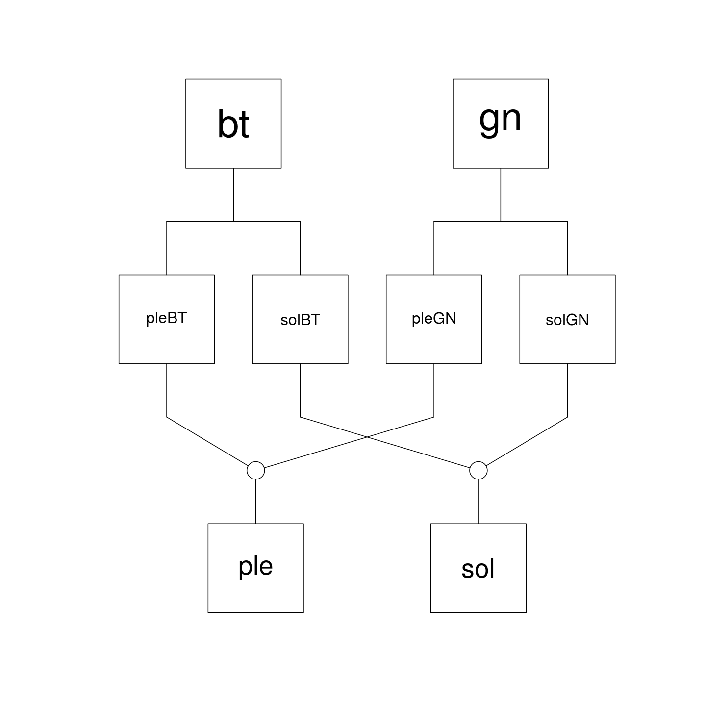
We project as normal:
test <- fwd(object = biols, fishery = flfs, control = ctrl)We check out the total plaice catch from both fisheries, and also the relative sole catch:
catch_ple_bt <- catch(test[["fisheries"]][["bt"]][["pleBT"]])[,
    ac(years)]
catch_ple_gn <- catch(test[["fisheries"]][["gn"]][["pleGN"]])[,
    ac(years)]
catch_sol_bt <- catch(test[["fisheries"]][["bt"]][["solBT"]])[,
    ac(years)]
catch_sol_gn <- catch(test[["fisheries"]][["gn"]][["solGN"]])[,
    ac(years)]
catch_ple_bt + catch_ple_gn
## An object of class "FLQuant"
## , , unit = unique, season = all, area = unique
##
## year
## age 2 3 4 5
## all 2e+05 2e+05 2e+05 2e+05
##
## units: NAcatch_sol_bt/catch_sol_gn## An object of class "FLQuant"
## , , unit = unique, season = all, area = unique
##
## year
## age 2 3 4 5
## all 0.8 0.8 0.8 0.8
##
## units: NA10.3 Setting a joint effort limit
The corresponding individual effort from each FLFishery is in the above example:
effort(test[["fisheries"]][["bt"]])[, ac(years)]## An object of class "FLQuant"
## , , unit = unique, season = all, area = unique
##
## year
## quant 2 3 4 5
## all 0.63774 0.53341 0.48727 0.46268
##
## units: NAeffort(test[["fisheries"]][["gn"]])[, ac(years)]## An object of class "FLQuant"
## , , unit = unique, season = all, area = unique
##
## year
## quant 2 3 4 5
## all 1.5638 1.7128 1.9431 2.1127
##
## units: NAWe can set an additional constraint of maximum total effort of both fisheries, a joint target set at the FLFishery level. Here we have two efforts to solve (one from each FLFishery) which means that we must have two subtargets in each target in each time step (year). This means that if we want to introduce a maximum constraint on effort we must also include a second subtarget. Constraint targets (maximum and minimum targets) are solved after non-constraint targets. This means that if a target has a constraint subtarget then all the other subtargets of that target must also be constraints. We can set up a dummy constraint that is never triggered just to make up the numbers (however, it cannot be a separate minimum effort target for the two fishery objects).
total_max_effort <- 2
years <- 2:5
# targets + constraints (max effort, min biomass)
ctrl <- fwdControl(list(year = years, quant = "catch", value = total_ple_catch,
    fishery = G("bt", "gn"), catch = G("pleBT", "pleGN")), list(year = years,
    quant = "catch", value = 0.8, fishery = "bt", catch = "solBT",
    relYear = years, relFishery = "gn", relCatch = "solGN"),
    list(year = years, quant = "effort", max = total_max_effort,
        fishery = G("bt", "gn")), list(year = years, quant = "biomass_end",
        min = 1, biol = "ple"), FCB = fcb)
ctrl
## An object of class "fwdControl"
## (step) year quant relYear relFishery relCatch
## 1 2 catch NA <NA> <NA>
## 2 2 catch 2 gn solGN
## 3 2 effort NA <NA> <NA>
## 4 2 biomass_end NA <NA> <NA>
## 5 3 catch NA <NA> <NA>
## 6 3 catch 3 gn solGN
## 7 3 effort NA <NA> <NA>
## 8 3 biomass_end NA <NA> <NA>
## 9 4 catch NA <NA> <NA>
## 10 4 catch 4 gn solGN
## 11 4 effort NA <NA> <NA>
## 12 4 biomass_end NA <NA> <NA>
## 13 5 catch NA <NA> <NA>
## 14 5 catch 5 gn solGN
## 15 5 effort NA <NA> <NA>
## 16 5 biomass_end NA <NA> <NA>
## fishery catch biol min value max
## bt, gn pleBT, pleGN <NA> NA 200000.000 NA
## bt solBT <NA> NA 0.800 NA
## bt, gn NA <NA> NA NA 2.000
## NA NA ple 1.000 NA NA
## bt, gn pleBT, pleGN <NA> NA 200000.000 NA
## bt solBT <NA> NA 0.800 NA
## bt, gn NA <NA> NA NA 2.000
## NA NA ple 1.000 NA NA
## bt, gn pleBT, pleGN <NA> NA 200000.000 NA
## bt solBT <NA> NA 0.800 NA
## bt, gn NA <NA> NA NA 2.000
## NA NA ple 1.000 NA NA
## bt, gn pleBT, pleGN <NA> NA 200000.000 NA
## bt solBT <NA> NA 0.800 NA
## bt, gn NA <NA> NA NA 2.000
## NA NA ple 1.000 NA NAtest <- fwd(object = biols, fishery = flfs, control = ctrl)What happened? First we take a look at the effort. We can see that the total effort has been constrained by the effort limit.
# Check that all the target pairs in each year solved
test[["flag"]]
## [,1]
## [1,] 1
## [2,] 1
## [3,] 1
## [4,] 1
## [5,] 1
## [6,] 1
## [7,] 1
## [8,] 1# Look at effort
effort_bt <- (test[["fisheries"]][["bt"]]@effort)[, ac(years)]
effort_gn <- (test[["fisheries"]][["gn"]]@effort)[, ac(years)]
effort_bt + effort_gn## An object of class "FLQuant"
## , , unit = unique, season = all, area = unique
##
## year
## quant 2 3 4 5
## all 2 2 2 2
##
## units: NAConsequently the catch targets have not been hit
catch_ple_bt <- catch(test[["fisheries"]][["bt"]][["pleBT"]])[,
    ac(years)]
catch_ple_gn <- catch(test[["fisheries"]][["gn"]][["pleGN"]])[,
    ac(years)]
catch_sol_bt <- catch(test[["fisheries"]][["bt"]][["solBT"]])[,
    ac(years)]
catch_sol_gn <- catch(test[["fisheries"]][["gn"]][["solGN"]])[,
    ac(years)]
catch_ple_bt + catch_ple_gn
## An object of class "FLQuant"
## , , unit = unique, season = all, area = unique
##
## year
## age 2 3 4 5
## all 200051 199957 199884 199863
##
## units: NAcatch_sol_bt/catch_sol_gn## An object of class "FLQuant"
## , , unit = unique, season = all, area = unique
##
## year
## age 2 3 4 5
## all 1.0455 1.0527 1.2195 1.3094
##
## units: NA11 References
Scott, F. and Mosqueira, I. 2016. Bioeconomic Modelling for Fisheries; EUR 28383 EN; doi:10.2788/722156